Authors:
(1) Luyuan Peng, Acoustic Research Laboratory, National University of Singapore;
(2) Hari Vishnu, Acoustic Research Laboratory, National University of Singapore;
(3) Mandar Chitre, Acoustic Research Laboratory, National University of Singapore;
(4) Yuen Min Too, Acoustic Research Laboratory, National University of Singapore;
(5) Bharath Kalyan, Acoustic Research Laboratory, National University of Singapore;
(6) Rajat Mishra, Acoustic Research Laboratory, National University of Singapore.
Table of Links
IV Experiments, Acknowledgment, and References
II. METHOD


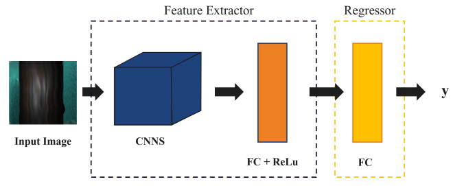
We implement two different architectures. The first uses pretrained deep convolutional neural networks (DCNN) to extract features from the input images. The resulting feature map is then passed to an affine regressor consisting of dense neural layers to output a 7-dimensional pose vector estimates. The second architecture adds an additional LSTM layer between the DCNN and affine regressor to perform dimensionality reduction by assessing the spatial structure of the image. This is done by four LSTMs which parse the DCNN-output feature map in different directions starting at each of the four image corners to process the spatial trends, and compress it into lower-dimensional information which is easier processed by the affine regressor.
The input images used in the training are rescaled to 256×256 pixels before cropping into a 224×224 feature input using centre cropping. To speed up training, the images are normalized by the mean and standard deviation of the images. The poses are also normalized to lie within [-1, 1].


This paper is available on arxiv under CC BY 4.0 DEED license.

